We arrived to the island after the ferry trip and we see ourselves in need of transportation to the nearest airport. Fortunately there’s a shuttle bus service between the sea port and the airport that could take us there.
Day 13 is a wonderful mathematical puzzle, following the theme of modular arithmetic of the previous one. Let’s dive into it as there some surprises with the numeric limits on Power BI.
If you want to follow along please download AdventOfCode2020.pbit and check Day 1 post for instructions.
Part 1
To solve the first part of the puzzle we have to find the earliest time we could depart on a bus. The first line of our input is a numeric value representing a timestamp and the second line the ids of the bus on service. There’s some ‘x’ characters amidst the bus ids that represent out of service bus that are of no interest to find the answer.
The timestamp marks the moment after we can depart aboard of the buses and each bus id represents the duration of the trip. So a bus with id 7, departs each 7 minutes \([0, 7, 14, 21,…]\).
Now that we understand the rules we need to find which bus leaves first after a certain timestamp, calculate the difference between the two timestamps and multiply that value by the bus id.
This looks like a nice problem to solve using some DAX.
But first we need to import our data.

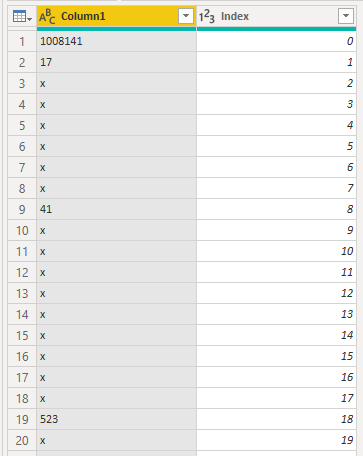
Split by delimiter, add an index:

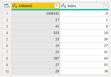
And remove those useless ‘x’s:

With our data ready, a way to solve this problem is to subtract to the bus id the remainder of the division of the timestamp by the bus id. The smallest difference will be the answer. Taking the sample data we can test our algorithm:
\[7 - (939 \bmod 7) = 6 \] \[13 - (939 \bmod 13) = 10 \] \[59 - (939 \bmod 59) = 5 \] \[31 - (939 \bmod 31) = 22 \] \[19 - (939 \bmod 19) = 11 \]
The smallest is 5 and multiplying by 59 we have 295.
Translating this idea to DAX, we create a variable to store the
timestamp in our file and on variable tt the remaining rows of the
table. In our return value, we calculate the difference between the
bus id and the remainder of the division of the timestamp by the bus
ids. Then we sort that value by ascending order and pick the first row
using the TOPN function.
Multiplying the difference by the bus id returns the answer for the first part of our puzzle.
VAR earliestTimestamp =
    CALCULATE (
        MAX ( input_day_12_sample[BusId] ),
        input_day_12_sample[Index] = 0
    )
VAR tt =
    FILTER (
        input_day_12_sample,
        input_day_12_sample[BusId] <> earliestTimestamp
    )
RETURN
    SELECTCOLUMNS (
        TOPN (
            1,
            ADDCOLUMNS ( tt, "Mod", [BusId] - MOD ( earliestTimestamp, [BusId] ) ),
            [Mod], ASC
        ),
        "Part 1", [BusId] * [Mod]
    )
Part 2
Now the fun begins. We need to find the first timestamp from which the first bus on the list departs and in the subsquent timestamp the second one departs and so on until the end of the list. An ‘x’ in the schedule means that there are no departures in that minute.
If you check the provided example:
7,13,x,x,59,x,31,19

| timestamp | bus departure |
+-----------+---------------+
| t         |        7      |
| t+1       |        13     |
| t+4       |        59     |
| t+6       |        31     |
| t+7       |        19     |
How do we find that t? A possibility would be to try and apply some
brute force testing incrementing numbers until we find one which is
multiple of seven, will have a remainder of one when divided by 13, 4
when divided by 59, 6 when divided by 31 and 7 when divided by 19. But
reading through the text on the puzzle we see that brute forcing will
be impractical as the numbers can be really big.
A more doable approach is being smart about the increment steps. We would start with increments of size 7 plus 1, the delay, and when a number that’s divisible by 13 is found we would increment the loop step by 13*7. An example to illustrate the algorithm:
time stamp:   7     loop interval:  7      check: ( 7+1) mod 13 == 0? FALSE
time stamp:  14     loop interval:  7      check: (14+1) mod 13 == 0? FALSE
...
time stamp:  78     loop interval:  7      check: (78+1) mod 13 == 0? TRUE
time stamp: 169     loop interval: 91      check: (91+4) mod 59 == 0? FALSE
...
And we will keep going till the last bus, getting our answer. This will work but there’s a more elegant of solving the problem by using the method known as the “Chinese Remainder Theorem”. We are in conditions to apply it because the examples and the input file are composed of only prime numbers.
I’ll try my best to show you how we can use the theorem to solve this
and implement the code in Power Query.
We want a number that will satisfy the conditions:
\begin{align*} x &\equiv 0 \:(\bmod 7) \\\ x &\equiv 12 \:(\bmod 13) \\\ x &\equiv 55 \:(\bmod 59) \\\ x &\equiv 25 \:(\bmod 31) \\\ x &\equiv 12 \:(\bmod 19) \\\ \end{align*}
First step is to calculate \(N\).
\begin{align*} N &= 7 * 13 * 59 * 31 * 19\\\ &= 3162341 \end{align*}
Then each of our \(Ni\):
\begin{align*} N_1 &= N/7\ \; =& 451\,763\\\ N_2 &= N/13 =& 243\,257\\\ N_3 &= N/59 =& 53\,599 \\\ N_4 &= N/25 =& 102\,011\\\ N_5 &= N/12 =& 166\,439\\\ \end{align*}
After we calculate the inverse \(mod\) for each of our values:
\begin{align*} 0x_1 &\equiv 1 (\bmod 7) \\\ 12x_2 &\equiv 1 (\bmod 13) \\\ 55x_3 &\equiv 1 (\bmod 59) \\\ 25x_4 &\equiv 1 (\bmod 31) \\\ 12x_5 &\equiv 1 (\bmod 19) \\\ \end{align*}
We will get:
\begin{align*} 2x_1 &\equiv 1 (\bmod 7) \\\ 1x_2 &\equiv 1 (\bmod 13) \\\ 35x_3 &\equiv 1 (\bmod 59) \\\ 3x_4 &\equiv 1 (\bmod 31) \\\ 18x_5 &\equiv 1 (\bmod 19) \\\ \end{align*}
Putting our data in a table, we just have to sum the products and will have our solution:
| \(bi\) | \(Ni\) | \(x_i\) | \(b_iN_ix_i\) |
|---|---|---|---|
| 0 | 451763 | 2 | 0 |
| 12 | 243257 | 1 | 2919084 |
| 55 | 53599 | 35 | 103178075 |
| 25 | 102011 | 3 | 7650825 |
| 12 | 166439 | 18 | 35950824 |
\begin{equation} x = 0+2\,919\,084+103\,178\,075+7\,650\,825+35\,950\,824 = 149\,698\,808\\\ \\\ x \equiv 149\,698\,808\: (\bmod 3\,162\,341)\\\ \\\ x \equiv \mathbf{1\,068\,781}\: (\bmod 3\,162\,341) \end{equation}
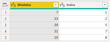
We got to the result. So it seems we are ready to implement this
algorithm in Power BI. Starting from this table:

- \(N\)
List.Product([Modulus]) - \(b_i\)
Number.Mod([Modulus] - Number.Mod([Index]-1,[Modulus]), [Modulus]) - \(N_i\)
N / [Modulus] - \(x_i\)
fnInvertMod([Ni], [Modulus]) - \(b_iN_ix_i\)
List.Product({[Remainders], [Ni], [Xi]}, Precision.Decimal)
Here’s the fnInvertMod code that implements the Extended Euclidian Algorithm:
fnInvertMod = (ni as number, modulus as number) =>
let
    fnRecInvertMod =
        (a as number, b as number, x as number, y as number) =>
            if b = 0
            then if x < 0 then x + modulus else x
            else @fnRecInvertMod(b, Number.Mod(a, b), y, x - y * Number.IntegerDivide(a,b))
in
    fnRecInvertMod(ni, modulus, 1, 0)
What you are seeing here is a recursive function. These functions in
Power Query have a the @ character on the recursive call which
makes them easy to spot. They are an alternative to the list looping
functions we have been using while solving the puzzles. Beware as they
can be slow or can fault when the recursive tree is long.
Another interesting thing you can see is the use of the
Precison.Decimal parameter when calculating the product. This is
need because by default Power Query works with double precision
which conforms with IEEE standard. You can check more details on this
Power Query M Primer (Part 7): Types—Numbers by Ben Gribaudo. To shown
you what I mean, when working with the full set of values:


Not forcing the precision causes these differences and you should be
aware when working with such large numbers of the limits of Power
BI.
And finally our answer can be obtained by doing:
Number.Mod(List.Sum([BiNiXi],Precision.Decimal),N,Precision.Decimal)
Conclusion
I have had a lot fun with this one. Really liked to use some Math to
solve problems instead of going full brute force mode on. Also was a
great exploration on the numeric limits to the calculations you can
use on Power BI. The part 2 of this puzzle was impossible to solve
by using DAX due to the numeric rounding. There’s an implicit
conversion from ‘Whole Number’ to ‘Decimal Number’ when dividing
numbers that causes the imprecision.
(https://docs.microsoft.com/en-us/power-bi/connect-data/desktop-data-types#implicit-and-explicit-data-type-conversion-in-dax-formulas)
Also be aware due to JavaScript limitations visuals are limited to
numbers below 9 007 199 254 740 991 (16 digits long). Here’s what you
can see when trying to see a number bigger than the limit:

And here’s the real number as shown with Power Query:

I’ll leave you with an excellent read about this theme - Choosing Numeric Data Types in DAX article from Marco Russo. It can help you avoid issues when designing your data models.
Have fun!!
